The Margin Makers

In the ever-expanding landscape of machine learning, Support Vector Machines (SVMs) stand out as a mathematically elegant and effective method for classification and regression tasks. Despite the rise of deep learning models in recent years, SVMs remain a staple in the toolbox of data scientists due to their strong theoretical foundations [1], versatility, and impressive performance on small to medium-sized datasets.

This article delves into the core concepts behind SVMs, how they work, their mathematical underpinnings, advantages and limitations, and some of the key areas where they continue to be applied successfully.

1. The Classification Problem

At the heart of machine learning lies the problem of classification: given an input, can we assign it to one of several predefined categories? Formally, this involves finding a function that maps feature vectors x∈{R}^n to discrete labels y∈{−1,+1} (in the binary case).

The goal is to find a decision boundary that separates classes with the highest possible accuracy. For linearly separable data, many boundaries may achieve perfect separation, but which one should we choose?

SVMs address this by finding the maximum-margin hyperplane, the one that maximizes the distance between the closest points of each class and the boundary itself.

2. Intuition Behind SVMs

At its core, the intuition behind Support Vector Machines revolves around geometry and optimization. The main idea is not just to separate the data into classes, but to do so in the most confident way possible.

2.1 A Geometric Perspective

Imagine a simple case: a 2D plane where each data point belongs to one of two classes, say red circles and blue squares. There are many lines you could draw that cleanly separate these two classes. The key question SVM answers is: Which line is best?

SVM chooses the optimal separating hyperplane, defined as the one that maximizes the margin, the distance between the hyperplane and the closest data points from each class.

📌 Definition: Margin

The margin is the distance between the decision boundary and the nearest data points of each class. Maximizing this distance is essential because:

• It reduces the model’s sensitivity to small fluctuations in the data.
  

• It improves generalization to unseen data.
  

• It helps prevent overfitting, especially in high-dimensional settings.
  

This optimal boundary is known as the maximum-margin hyperplane.

2.2 Why Support Vectors Matter

Once the maximum-margin hyperplane is identified, it turns out that only a few data points determine its position. These are the support vectors, the samples that lie exactly on the edge of the margin.

All other data points — even if they are correctly classified — do not affect the decision boundary at all. You could remove them, and the result would be the same. This leads to two key insights:

• Sparsity: The model depends only on a subset of the data, which makes it efficient for prediction.
  

• Interpretability: Support vectors are often the “hard cases” — borderline examples — and analyzing them can provide insights into the problem.
  

📉 Example (Visual Figure Suggestion)

Imagine this diagram:

Visualization of a linear Support Vector Machine (SVM). The green dashed line represents the decision boundary, while the shaded region illustrates the margin 𝑀. The circled data points are the support vectors — the critical elements that define the margin. Points outside the margin do not influence the position of the separating hyperplane.

Only the closest instances (support vectors) influence the boundary.

2.3 SVM vs Other Classifiers

Other classifiers, like logistic regression or decision trees, attempt to minimize classification error. This can result in boundaries that are close to some data points and highly sensitive to outliers.

SVM takes a different approach:

• It doesn’t just aim to get every point right.
  

• It aims to make the most confident separation, even if that means allowing for some misclassifications (in the soft-margin variant).
  

• This confidence is mathematically encoded as margin maximization.
  

2.4 What If the Data Isn’t Linearly Separable?

SVMs are still applicable when no straight line (or hyperplane) can perfectly separate the classes. Two strategies are employed:

• Slack variables: Allow some misclassifications in exchange for a larger overall margin.
  

• Feature transformation via kernels: Map the data to a higher-dimensional space where a linear separator does exist.
  

This ability to find a maximum-margin separator even in transformed spaces is a key strength of SVMs.

📉 Example (Visual Suggestion)

To understand how the kernel trick enables SVMs to classify non-linearly separable data, consider the following example:

In the following figure, we plot a set of points arranged in two concentric circles. Each circle corresponds to a different class. Clearly, there is no straight line in 2D space that can separate these two classes without error; the problem is not linearly separable.

Two concentric circles representing a non-linearly separable dataset in 2D. No straight line can separate the two classes without error

However, notice that the only difference between the two classes is their distance from the origin. This inspires a transformation: instead of working in the 2D plane (x, y), we map each point to a new 3D space using the function:

ϕ(x,y)= (x, y, x^2 + y^2)

In the next figure, we visualize this transformation. Now the inner circle is mapped to a smaller height and the outer circle to a greater height along the new axis z=x^2 + y^2. The two classes become separable by a flat plane in this 3D space.

The same data mapped to 3D using the transformation ϕ. The classes now lie on distinct horizontal planes, making them linearly separable.

This is the essence of the kernel trick: instead of manually computing the mapping ϕ, SVMs use a kernel function (such as the RBF kernel) to compute inner products in the high-dimensional space directly, enabling linear separation in transformed feature spaces while working efficiently in the original input space.

2.5 Summary of the Intuition

• Maximize the margin: A wider margin usually implies better generalization.
  

• Use only support vectors: These are the most informative points.
  

• Separate confidently, not just correctly: SVM prioritizes robustness.
  

• Apply kernels when necessary: Transform the data instead of fitting complex models.
  

This intuition — elegant and grounded in geometry — is what makes SVMs simultaneously powerful and conceptually satisfying[2].

3. The Mathematics of SVM

3.1 The Hard-Margin SVM

For linearly separable data, SVM solves the following optimization problem:

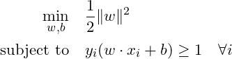
Where:

• w is the weight vector perpendicular to the hyperplane.
  

• b is the bias term.
  

• x_i​ are the input vectors.
  

• y_i ∈ {−1,+1} are the class labels.

  
  

The constraint ensures that all points lie on the correct side of the margin.

3.2 The Soft-Margin SVM

Real-world data is rarely perfectly separable. To accommodate noise and overlapping classes, soft-margin SVM introduces slack variables [4] ξ_i​ to allow some points to fall within or even across the margin:

The parameter CCC controls the trade-off between maximizing the margin and minimizing classification errors.

4. Non-Linear SVMs and the Kernel Trick

4.1 The Need for Non-Linear Boundaries

Many real-world problems involve data that is not linearly separable, even with slack variables. SVMs handle this elegantly by projecting the data into a higher-dimensional space where a linear separation is possible.

This transformation is enabled by the kernel trick.

4.2 What Is a Kernel?

A kernel is a function K(x_i, x_j) that computes the inner product between the images of x_i and x_j in a high-dimensional space, without ever computing the mapping explicitly. Popular kernels include:

• Linear kernel: K(x_i, x_j) = x_i * x_j
  

• Polynomial kernel: K(x_i, x_j) = (x_i * x_j + 1)^d
  

• RBF (Gaussian) kernel: K(xi,xj)=exp(−γ ∥xi​−xj​∥^2)
  

• Sigmoid kernel: Related to neural networks
  

The result is that SVMs can learn complex, non-linear decision boundaries while still retaining convex optimization guarantees.

5. Support Vectors and Decision Function

At the heart of an SVM model lie the support vectors — the data points that are closest to the decision boundary and therefore most critical in defining it. Once the optimal hyperplane is determined during training, only these support vectors are used to construct the final decision function.

This is one of the most elegant aspects of SVMs: the model complexity depends not on the entire dataset but only on a subset of examples. These support vectors are the only points that influence the position and orientation of the separating hyperplane.

5.1 The Decision Function

After training, the SVM classifier makes predictions using the following decision function:

Where:

• x_i​ are the support vectors.
  

• yi∈{−1,+1} are their class labels.
  

• α_i​ are Lagrange multipliers determined during training.
  

• K(x_i, x) is the kernel function, which defines the similarity between the test point x and each support vector.
  

• b is the bias term.
  

Only support vectors have non-zero α_i​, which is why the summation is limited to them.

This formula makes the prediction process highly efficient and scalable, particularly when the number of support vectors is small compared to the overall dataset.

5.2 Interpretability and Sparsity

One of the practical benefits of SVMs is sparsity: most data points do not influence the model at all once training is complete. This property has two important implications:

• Efficiency at inference time: Since only support vectors are used, predictions are faster and require less memory than other methods like k-NN.
  

• Interpretability: Support vectors can be inspected to understand borderline or ambiguous cases in the data; they are the most "difficult" points to classify and thus often informative.
  

In real-world problems, especially in high-dimensional settings, this selective reliance on key examples makes SVMs a robust choice even when data is limited.

6. SVMs for Regression: Support Vector Regression 

Although SVMs are best known for classification, they can also be adapted for regression tasks through a technique called Support Vector Regression (SVR).

The core idea behind SVR is to find a function that approximates the target values while allowing for some tolerance. Specifically, SVR seeks to fit a function that deviates from the actual target y_i​ by no more than a fixed margin ϵ. Deviations within this “ε-insensitive zone” are not penalized.

Support Vector Regression (SVR) using an RBF kernel. The dark blue line represents the predicted regression function. The light blue shaded area shows the ε-insensitive tube, within which prediction errors are not penalized. Data points outside this tube act as support vectors and influence the model.

To handle points that fall outside this zone, slack variables are introduced, similar to the soft-margin classification case. The optimization problem balances two goals:

• Keeping the function as flat as possible (minimizing model complexity).
  

• Minimizing the number and magnitude of errors beyond ϵ.
  

SVR retains many advantages of standard SVMs: it’s robust to outliers, works well in high-dimensional spaces [3], and can handle non-linear patterns via kernel functions like the RBF kernel.

Applications of SVR include time series forecasting, financial modeling, and energy demand prediction, cases where precision and robustness are more important than interpretability.

7. Strengths and Limitations

7.1 Strengths

• Effective in high-dimensional spaces: Especially useful when the number of dimensions exceeds the number of samples.
  

• Robust to overfitting: Particularly when using the maximum-margin principle.
  

• Flexible: Thanks to the kernel trick.
  

• Well-defined optimization: Always converges to a global minimum due to convexity.
  

7.2 Limitations

• Not scalable to very large datasets: Training complexity is typically O(n^2) to O(n^3).
  

• Requires careful tuning: Hyperparameters like C, kernel choice, and kernel parameters greatly influence performance.
  

• Less interpretable than linear models: Especially with non-linear kernels.

8. Applications of SVMs

8.1 Bioinformatics

SVMs have been widely used for gene expression analysis, protein classification, and disease prediction due to their ability to handle high-dimensional data.

8.2 Text Classification

Tasks like spam detection, sentiment analysis, and document categorization have benefited from SVMs because of their performance on sparse, high-dimensional feature spaces.

8.3 Image Recognition

Before deep learning became dominant [6], SVMs were state-of-the-art for tasks such as digit recognition (e.g., MNIST) and face detection (e.g., using HOG features).

8.4 Finance

SVMs are employed for credit scoring, fraud detection, and stock price prediction, often in combination with other models.

9. Comparison with Other Algorithms

Feature	SVM	Logistic Regression	Decision Trees	Neural Networks
Model Complexity	Moderate	Low	Low to High	High
Handles Non-linearity	Yes (with kernels)	No	Yes	Yes
Scalability	Moderate (not ideal for big data)	High	High	High
Interpretability	Low (esp. with kernels)	High	Moderate to High	Low
Training Time	High (especially with kernels)	Low	Low to Moderate	High

10. Best Practices and Practical Tips

• Feature Scaling is crucial: SVMs are sensitive to the scale of input features. Always apply normalization or standardization.
  

• Use cross-validation: To select the best combination of C, kernel, and other hyperparameters.
  

• Start simple: Begin with a linear kernel. Only try non-linear ones if linear SVM performs poorly.
  

• Reduce dimensionality if needed: For very high-dimensional datasets, PCA[5] can help reduce training time.
  

Conclusion

Support Vector Machines remain a cornerstone of classical machine learning. Their ability to handle high-dimensional data, combined with solid theoretical underpinnings, makes them a go-to method for a wide range of classification and regression problems.

Although modern deep learning methods have taken the spotlight in many areas, SVMs still shine in cases where data is limited, interpretability matters, or computational resources are constrained. Understanding how SVMs work, from the geometric intuition to the kernel trick and beyond, equips practitioners with a powerful tool for building intelligent systems.

References

1. Cortes, C., & Vapnik, V. (1995). Support-vector networks. Machine Learning, 20(3), 273–297.
   

2. Cristianini, N., & Shawe-Taylor, J. (2000). An Introduction to Support Vector Machines and Other Kernel-based Learning Methods. Cambridge University Press.
   

3. Hsu, C.-W., Chang, C.-C., & Lin, C.-J. (2016). A practical guide to support vector classification.
   

4. Scholkopf, B., & Smola, A. J. (2002). Learning with Kernels: Support Vector Machines, Regularization, Optimization, and Beyond. MIT Press.
   

5. Dimensionality Reduction: Linear methods, Transcendent AI

   
   

6. The Power of Convolutional Neural Networks, Transcendent AI